1.96/sqrt(100)
0.196
\(ε_t\) 가 \(W N(0, σ^2)\)를 따를 때, 다음과 같은 확률과정 모형에 대하여 각 물음에 답하고, 답에 대한 이유를 밝혀라.
\[(1 − B)^2(1 − B^{12})Z_t = (1 − 0.5B)ε_t\]
\(\{Z_t\}\)는 정상시계열인가?
비정상 시계열이다.
(교수님풀이)
특성함수 \(\Phi(B) = (1-B)^2(1-B^{12})=0\)을 만족하는 모든 근의 절대값이 1보다 큰 것은 아니기 때문에 \((B = 1, -1)\) 정상시계열이 아니다.
\(W_t = (1 − B)Z_t\)는 정상시계열인가?
비정상 시계열이다. 한 번 차분해도 계절 성분이 있는 비정상 시계열을 얻는다.
(교수님풀이)
\((1-B)(1-B^{12})W_t = (1-0.5B)\epsilon_t\)이다. 이 때 특성함수 \(\Phi(B) = (1-B)(1-B^{12}) = 0\)을 만족하는 모든 근의 절대값이 1보다 큰 것은 아니기 때문에 \((B=1, -1)\) 정상시계열이 아니다.
\(W_t = Z_t − 2Z_{t−1} + Z_{t−2}\)는 정상시계열인가?
\(W_t=(1-B)^2\)가 정상 시계열인가 묻는 문제이다. 비정상 시계열이다. 두 번 차분해도 계절 성분이 있는 비정상 시계열을 얻는다.
(교수님 풀이)
\(W_t = (1-B^{12})Z_t\)이고, \((1-B)^2 W_t = (1-0.5B) \epsilon_t\)이 된다. 특성함수 \(\Phi(B) = (1-B)^2W_t = 0\)을 만족하는 모든 근의 절대값이 1보다 큰 것은 아니기 때문에 \((B=1)\) 정상 시계열이 아니다.
\(W_t = Z_t − Z_{t−12}\)는 정상시계열인가?
\(W_t = (1-B^{12})\)이다. 비정상시계열이다. 추세 성분이 남아있다.
(교수님 풀이)
\(W_t = (1-B^{12})Z_t\)이고, \((1-B)^2 W_t = (1-0.5B)\epsilon_t\)이 된다. 특성함수 \(\Phi(B) = (1-B)^2 W_t = 0\)을 만족하는 모든 근의 절대값이 1보다 큰 것은 아니기 때문에 \((B=1)\) 정상시계열이 아니다.
\(W_t = (1 − B)^2(1 − B^{12})Z_t\)는 정상시계열인가?
정상 시계열이다.
(교수님 풀이)
\(W_t = (1-0.5B)\epsilon_t\)이고, \(W_t \sim MA(1)\)익 때문에 정상 시계열이다.
다음은 시계열자료 \(\{Z_t\}\)의 표본 크기 \(n\), 평균 \(\bar Z\), 표준편차 \(s_Z\), 그리고 시차 13까지의 SACF와 SPACF이다. 각 시계열자료를 잘 설명하는 모형은 무엇인지 식별하여라.
- \(AR(p):\) SACF이용
\[H_0: \rho_k = 0 vs. H_1: \rho_k \neq 0, k=1,2, \dots\]
- 유의수준 \(\alpha=0.05\)에서,
\[|\hat \rho_k| > 1.96 s.e.(\hat \rho_k), k \geq q+1\]
이면 귀무가설 기각, 단
\[s.e(\hat \rho_k) \approx \sqrt{\frac{1}{n}(1+ 2\rho_1^2 + \dots + 2\rho_q^2)}\]
- \(MA(q)\): SPACF이용
\[H_0: \phi_{kk} = 0 vs. H_1: \phi_{kk} \neq 0, k=1,2,\dots\]
- 유의수준 \(\alpha=0.05\)에서,
\[|\hat \phi_{kk}| > \dfrac{1.96}{\sqrt{n}}, k \geq p+1\]
이면 귀무가설 기각
\(n = 100, \bar Z = 24.75, s_Z = 9.27\)
| k | 1 | 2 | 3 | 4 | 5 | 6 | 7 | 8 | 9 | 10 | 11 | 12 | 13 |
|---|---|---|---|---|---|---|---|---|---|---|---|---|---|
| \(\hat ρ_k\) | -0.48 | -0.04 | -0.06 | 0.14 | -0.22 | 0.19 | -0.10 | -0.02 | 0.09 | -0.03 | -0.12 | 0.09 | 0.03 |
| \(\hat ϕ_{kk}\) | -0.48 | -0.24 | -0.21 | 0.01 | -0.20 | -0.01 | -0.05 | -0.15 | -0.04 | -0.06 | -0.04 | 0.02 | 0.06 |
\(\hat{s.e}(\hat \rho_k)\) 값을 구해주자
\(\hat{s.e}(\hat \rho_1) = \sqrt{\frac{1}{n}(1)}\)
\(\hat{s.e}(\hat \rho_2) \approx \sqrt{\frac{1}{n}(1+2\rho_1^2)}= \sqrt{\frac{1}{n}(1+2 \times 0.48^2)}\)
- ACF: 1차 이후 절단 형태 : MA(1)
- PACF: 1.96/ \(\sqrt{100}\) = 0.196이므로 3차 이후 절단 형태 : AR(3)
- 더 간단한 형태인 MA(1)모형 선택 (ACF는 1시차 이후 절단이고, PACF는 서서히 감소하는 형태이므로 MA(1)모형이 더 적당하다.)
\[Z_t = \mu + (1-\theta B) \epsilon_t, \epsilon_t \sim WN(0,\sigma^2_\epsilon)\]
MME를 생각하면
\[\hat \mu = \bar Z = 24.75\]
\[\gamma_0 = \frac{1}{100} \sum_{t=1}^{100}(Z_t - \bar Z)^2 = \frac{99}{100} s^2_Z = 85.074\]
\[\hat \rho_1 = \frac{-\theta}{1+\theta^2} \rightarrow \hat \theta = \frac{-1 \pm \sqrt{1-4\rho_1^2} }{2\hat \rho_1} = 0.75, 1.33 \rightarrow \hat \theta = 0.75 (\because |\theta| < 1)\]
\[\gamma_0 = \sigma_\epsilon^2 (1+\theta^2) \rightarrow \hat \sigma^2_\epsilon = \frac{\gamma_0}{1+\hat \theta^2} = 54.45\]
- 따라서 다음의 모형이 적절하다.
\[Z_t - 24.75 = \epsilon_t - 0.75 \epsilon_{t-1}, \epsilon_t \sim WN(0.54,45)\]
MA(1)모형
1.96/sqrt(100)시차 2부터는 0.196보다 작다. 즉 다 0이므로 무시하자..
\(n = 100, \bar Z = 25.56, s_Z = 3.85\)
| k | 1 | 2 | 3 | 4 | 5 | 6 | 7 | 8 | 9 | 10 | 11 | 12 | 13 |
|---|---|---|---|---|---|---|---|---|---|---|---|---|---|
| \(\hat ρ_k\) | 0.59 | 0.44 | 0.33 | 0.23 | 0.24 | 0.16 | 0.05 | 0.01 | -0.03 | -0.11 | -0.08 | -0.07 | 0.01 |
| \(\hat ϕ_{kk}\) | 0.59 | 0.13 | 0.04 | -0.02 | 0.12 | -0.05 | -0.12 | -0.03 | -0.01 | -0.13 | 0.06 | 0.04 | 0.13 |
MME를 생각하면
\[\hat \mu = \bar Z = 25.56\]
\[\gamma_0 = \frac{1}{100} \sum_{t=1}^{100}(Z_t - \bar Z)^2 = \frac{99}{100} s^2_Z = 14.674\]
\[\hat \phi = \hat \roh_1 = 0.59\]
\[\gamma_0 = \frac{\sigma^2_\epsilon}{1-\phi^2} \rightarrow \hat \sigma^2_\epsilon = \hat \gamma_0(1-\hat \rho_1^2) = 2.467\]
- 따라서 다음의 모형이 적절하다.
\[Z_t - 25.56 = 0.59(Z_{t-1} - 25.56) + \epsilon_t, \epsilon_t \sim WN(0, 2.467)\]
AR(1)모형
\(n = 99, \bar W = 19.02, s_w = 1.351,\) 단 \(W_k = (1 − B)Z_k\)
| k | 1 | 2 | 3 | 4 | 5 | 6 | 7 | 8 | 9 | 10 | 11 | 12 | 13 |
|---|---|---|---|---|---|---|---|---|---|---|---|---|---|
| \(\hat ρ_k\) | -0.44 | -0.05 | -0.01 | -0.03 | 0.12 | -0.15 | 0.15 | -0.04 | -0.10 | 0.09 | 0.08 | -0.07 | 0.06 |
| \(\hat ϕ_{kk}\) | -0.44 | -0.31 | -0.25 | -0.25 | -0.07 | -0.21 | -0.01 | 0.02 | -0.09 | -0.02 | 0.03 | -0.02 | 0.01 |
차분을 한 번 진행했다.
W가 MA(1)모형이다.
그리고 Z_k는 ARIMA(0,1,1)모형이다.
- MME를 생각하면
\[\hat \mu = \bar W = 19.02\]
\[\gamma_0 = \frac{1}{99} \sum_{t=1}^{99}(W_t - \bar W)^2 = \frac{98}{99} s^2_W = 1.807\]
\[\hat \rho_1 = \frac{- \theta}{1+\theta^2} \rightarrow \hat \theta = \frac{-1 \pm \sqrt{1-4\rho_1^2}}{2 \hat \rho_1} = 0.597, 1.676 \rightarrow \hat \theta = 0.597 (\because |\theta|<1)\]
\[\gamma_0 = \sigma^2_\epsilon (1+\theta^2) \rightarrow \hat \sigma^2_\epsilon = \frac{\gamma_0}{1+\hat \theta^2} = 1.332\]
- 따라서 다음의 모형이 적절하다.
\[(1-B)Z_t = 19.02 + \epsilon_t - 0.597 \epsilon_{t-1}, \epsilon_t \sim WN(0, 1.332)\]
두 시계열 \(X_t\)와 \(Y_t\)가 각각 다음과 같은 MA(1)모형을 따른다고 하자.
\[X_t = ε_t − θ_1ε_{t−1}, ε_t ∼ W N(0, σ^2_ε)\]
\[Y_t = a_t + θ_1a_{t−1}, a_t ∼ W N(0, σ^2_a)\]
\(Z_t = X_t + Y_t\)는 어떤 모형이 되겠는가? 만일, \(σ^2_ε = σ^2_a = σ^2\) 이라면 어떤 모형이 되겠는가? 그 이유를 자세히 설명하여라.
\(\epsilon_t^* \sim N(0,1)\)이라고 가정하자.
그러면
\(X_t = \sigma_\epsilon \epsilon_t^* - \theta_1 \sigma_\epsilon \epsilon_{t-1}^*\)
\(Y_t = a_t \epsilon_t^* + \theta_1 \sigma_a \epsilon_{t-1}^*\)
\(X_t + Y_t = (\sigma_\epsilon + \sigma_a ) \epsilon_t^* + (-\theta_1 \sigma_\epsilon + \theta_1 a_n) \epsilon_{t-1}^*\)$
\(\tilde \epsilon_t = {(\sigma_\epsilon + \sigma_a ) \epsilon_t^*}\)
= \(\tilde \epsilon_t + \dfrac{-\theta_1\sigma_\epsilon + \theta_1 \sigma_a}{\sigma_\epsilon + \sigma_a} \times (\sigma_\epsilon + \sigma_a) \times \epsilon_{t-1}^*\)
\(\tilde \epsilon_{t-1} = (\sigma_\epsilon + \sigma_a) \times \epsilon_{t-1}^*\)
= \(\tilde \epsilon_t +\dfrac{-\theta_1\sigma_\epsilon + \theta_1 \sigma_a}{\sigma_\epsilon + \sigma_a} \times \tilde \epsilon_{t-1}\)
\(\therefore Z_t = \tilde \epsilon_t + \tilde \theta_1 \tilde \epsilon_{t-1}\) 이 되므로 MA(1) 모형이 된다.
만일, \(σ^2_ε = σ^2_a = σ^2\) 이라면 위 식에서 분수의 \(\dfrac{-\theta_1\sigma_\epsilon + \theta_1 \sigma_a}{\sigma_\epsilon + \sigma_a}\) 분자값이 0이 되므로
\(Z_t^* = \tilde \epsilon_t\) 가 되므로 WN이 된다.
(교수님 풀이)
\(X_t + Y_t = Z_t = \epsilon_t + a_t - \theta_1 (\epsilon_{t-1} - a_{t-1})\)$ : MA모형같기두 하구?
우선 \(\{ \epsilon_t \}\)와 \(\{a_t \}\)에 대하여 \(Cov(\epsilon_i, a_j) = 0, \forall i, j\)가 성립함을 가정한다.
\(E(Z_t) =0\)
\(\gamma_0 = Var(Z_t) = \sigma^2_\epsilon + \sigma^2_a + \theta_1^2 \sigma_\epsilon^2 + \theta_1^2 \sigma^2_a = (1+\theta_1^2)(\sigma_\epsilon^2 + \sigma_a^2)\)
\(\gamma_1 = Cov(Z_t, Z_{t-1}) = Cov(\epsilon_t + a_t - \theta_1 (\epsilon_{t-1} - a_{t-1}), \epsilon_{t-1} + a_{t-1} - \theta_1(\epsilon_{t-2} - a_{t-2})) = - \theta_1 (\sigma_\epsilon^2 - \sigma_a^2)\)
\(\gamma_2 = Cov(Z_t, Z_{t-2}) = Cov(\epsilon_t + a_t - \theta_1 (\epsilon_{t-1} + a_{t-1}), \epsilon_{t-2} + a_{t-2} - \theta_1 (\epsilon_{t-3} + a_{t-3})) = 0\)
\(\gamma_k = 0, \forall k \geq 2\)
ACF가 1시차 이후로 절단된 형태이며, 따라서 MA(1)과 같은 성질이다.
PACF는 ACF에 의해 결정!(책 202P) 이는 MA(1)을 따른다고 할 수 있다.
그리고 \(\sigma_\epsilon = \sigma_a\)인 경우에는 \(\gamma_1=0\)이 되므로 \(\gamma_k=0, \forall k \geq 1\)이 된다. 따라서 백색잡음 과정이다.
(R실습). ex7 3.txt는 \(\{ε_t\}\)가 \(WN(0, 25)\)를 따를 때 확률과정 \[(1 − B^4)Z_t = (1 − 0.5B)ε_t\] 로부터 생성된 모의실험자료이다. 다음 물음에 답하여라. .
주기가 4인 계절성분이 있다.
계절차분을 했을 때 MA(1)모형이다.
z4 <- scan("ex7_3.txt")\(Z_t\) 의 시계열 그림을 그려라. 비성상성이 존재하는가? 존재한다면 비정상성분은 무엇이라고 생각하는가?
plot.ts(z4, main = "ex7_3")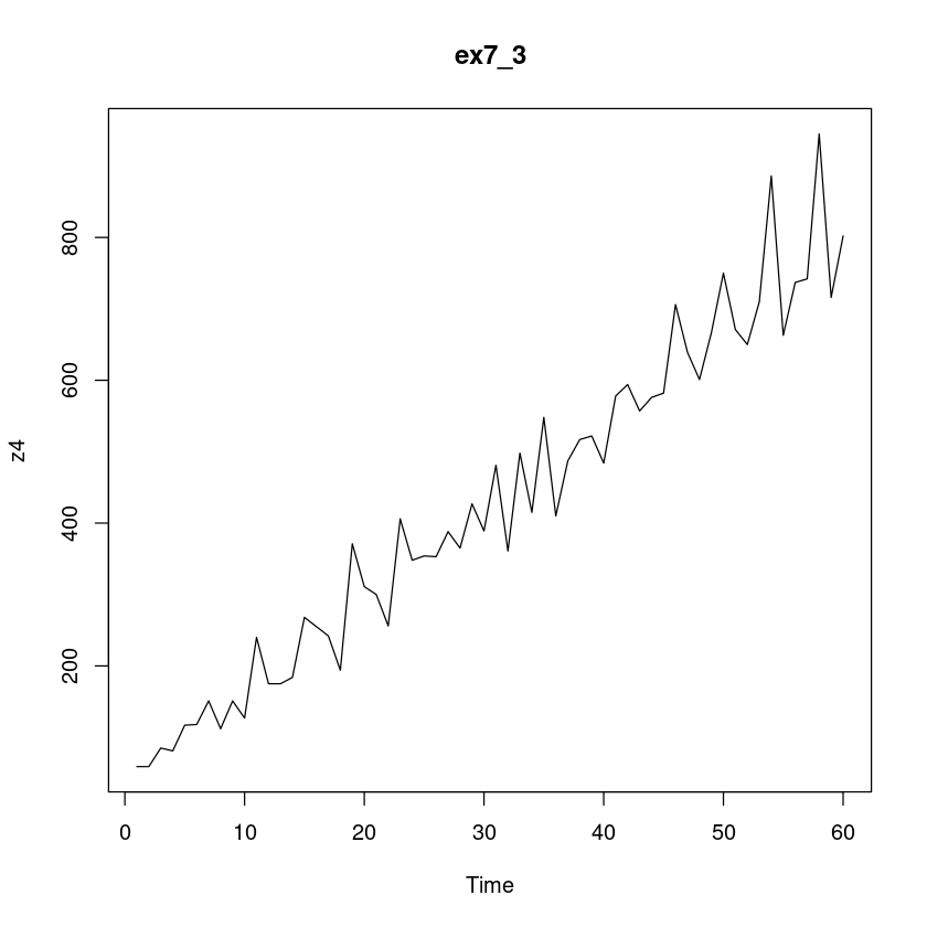
추세와 계절성분에 의한 비정상성이 존재하는 것으로 보인다.
1차 차분시계열 \((1 − B)Z_t\)의 시계열그림을 그려라. 계절성분에 의한 비정상성이 존재하는가? 존재한다면 계정성분을 제거하기 위하여 계절차분을 하여라.
options(repr.plot.width = 12, repr.plot.height = 10)
forecast::tsdisplay(diff(z4), lag.max=24)
Registered S3 method overwritten by 'quantmod':
method from
as.zoo.data.frame zoo
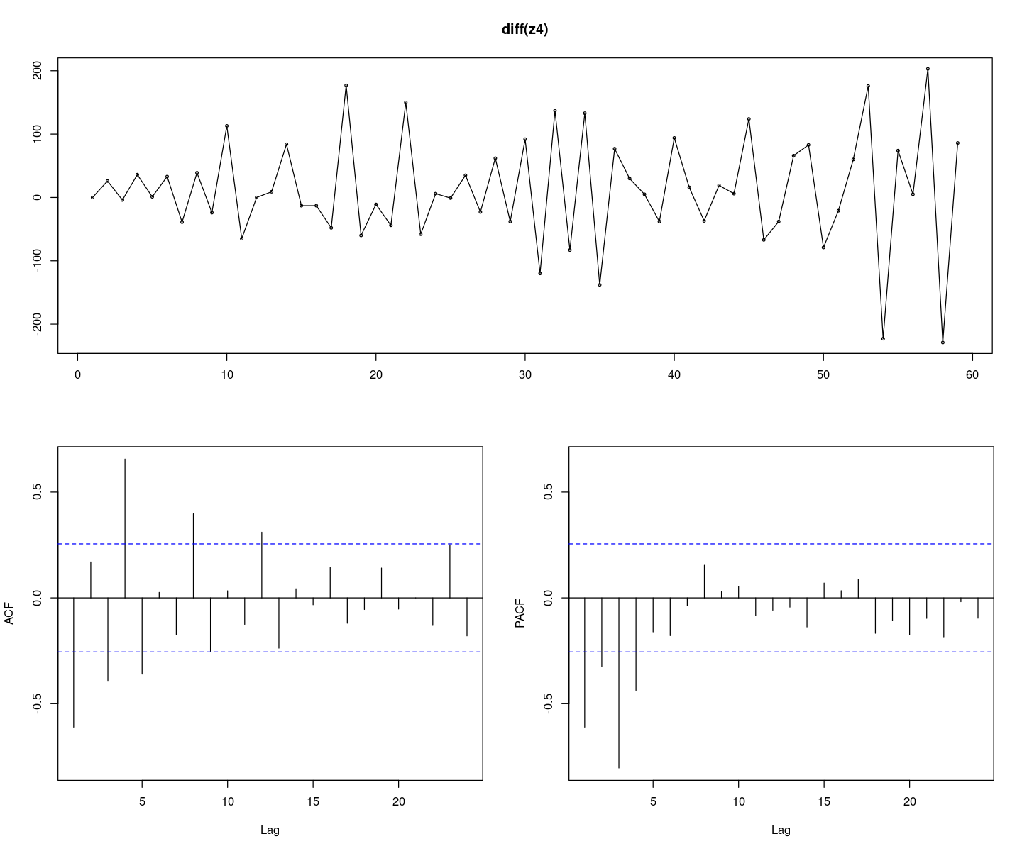
forecast::tsdisplay(diff(diff(z4),4), lag.max=24)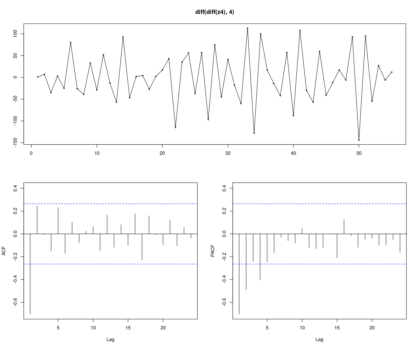
계절주기가 \(4\)인 계절차분된 시계열 \((1 − B^4)Z_t\)의 시계열을그림을 그려라. 비정상성이 존재하 는가?
z4_2 <- diff(z4, 4)
options(repr.plot.width = 12, repr.plot.height = 10)
forecast::tsdisplay(z4_2, lag.max=24)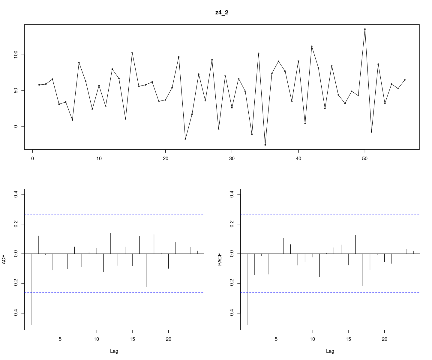
차분의 순서에 따라 결과가 달라짐에 주목하고 이에 대해 논하여라.
계절 차분을 먼저 진행하였고 추세가 없어짐을 볼 수 있다. 추세 차분을 먼저 진행하는 경우 계절 추세가 남을 수 있으니, 계절 차분을 먼저 진행해 주는 것이 좋다.
(R실습). ex7 4.txt는 \(\{ε_t\}\)가 \(W N(0, 25)\)를 따를 때 확률과정 \[(1 − B^4)(1 − B)Z_t = (1 − 0.5B)ε_t\] 로부터 생성된 모의실험자료이다. 다음 물음에 답하여라. .
\(Z_t\) 의 시계열 그림을 그려라. 비성상성이 존재하는가? 존재한다면 비정상성분은 무엇이라고 생각하는가?
z5 <- scan("ex7_4.txt")plot.ts(z5, main = "ex7_4")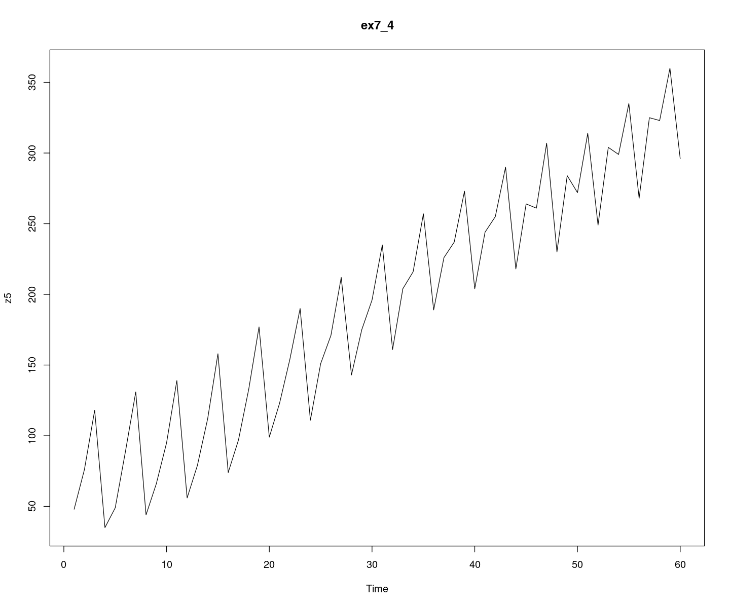
시도표를 확인 했을 때는 계절 성분이 있어 보이고, 시간에 따라 분산이 점점 작아 보인다.
1차 차분시계열 \((1 − B)Z_t\)의 시계열그림을 그려라. 계절성분에 의한 비정상성이 존재하는가?
options(repr.plot.width = 12, repr.plot.height = 10)
forecast::tsdisplay(diff(z5), lag.max=24)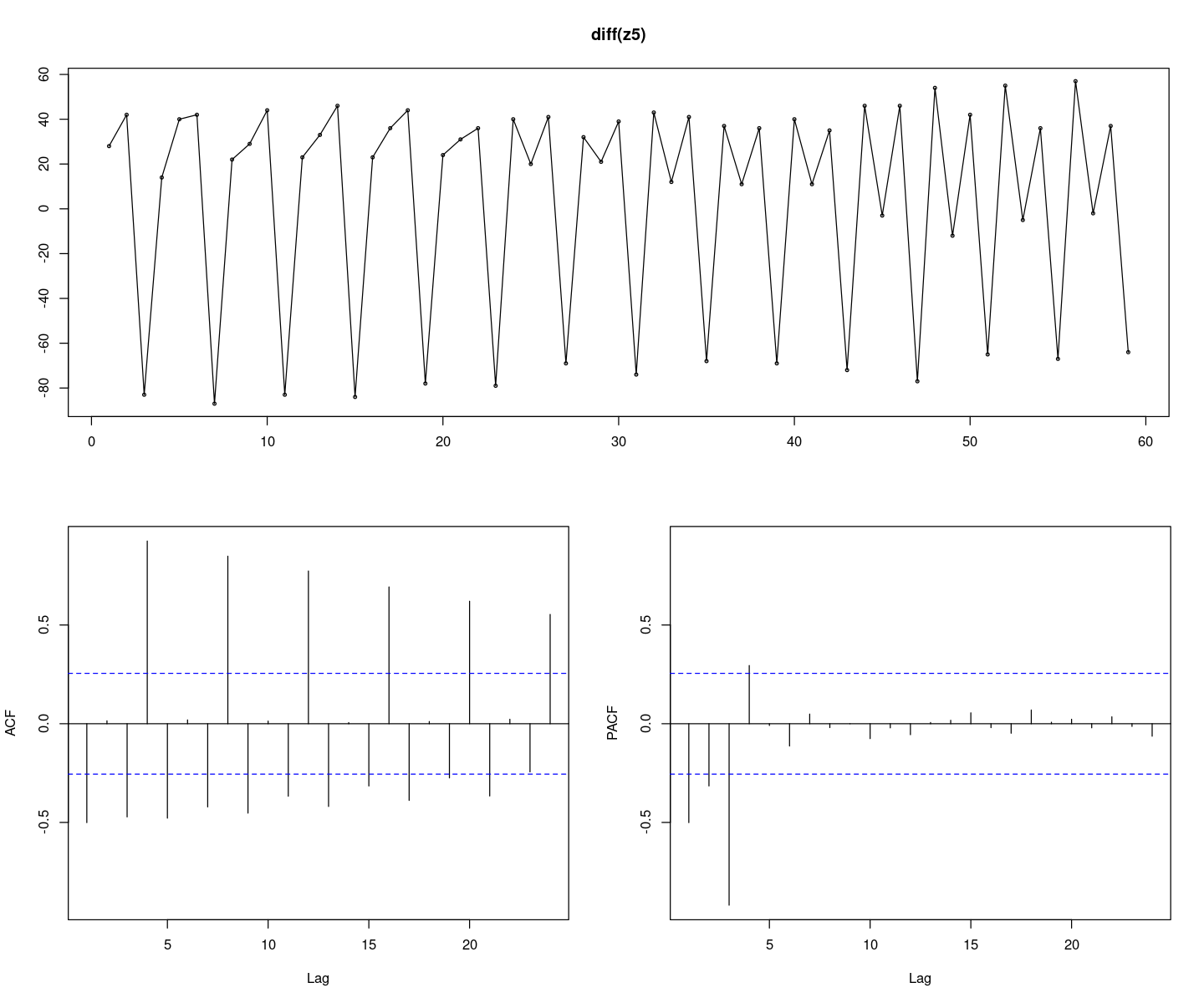
계절성분에 의해 ACF가 주기에 따라 들쭉 날쭉 하다. 비정상 시계열이다.
계절주기가 \(4\)인 계절차분된 시계열 \((1 − B^4)Z_t\)의 시계열을그림을 그려라. 비정상성이 존재하 는가? 존재한다면 비정상성분은 무엇이라 생각되는가?
z5_2 <- diff(z5, 4)
options(repr.plot.width = 12, repr.plot.height = 10)
forecast::tsdisplay(z5_2, lag.max=24)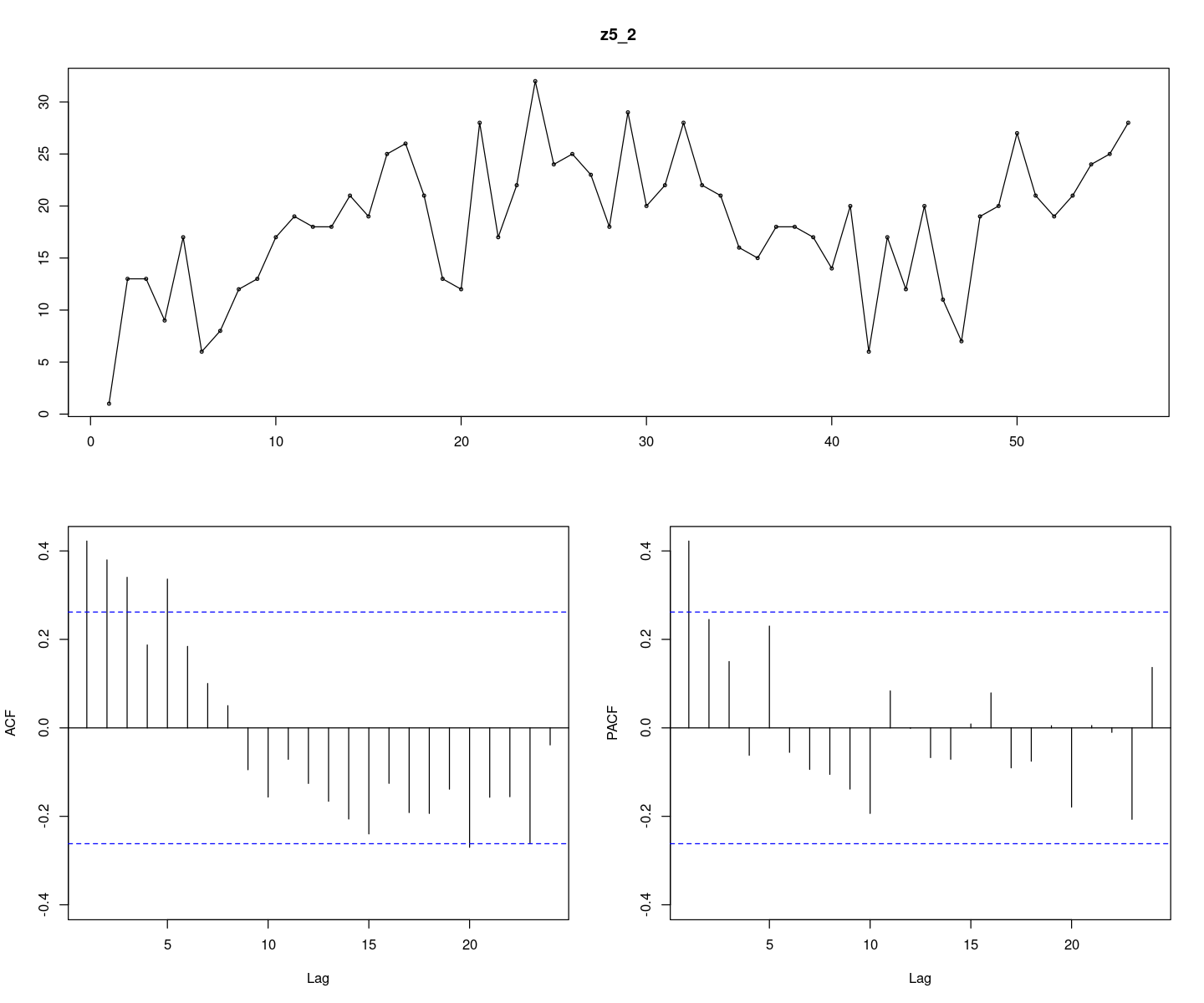
정상 시계열이다..(아마..)
1차 및 계절 차분 된 시계열 \((1 − B^4)(1 − B)Z_t\) 의 시계열그림을 그려라. 비정상성이 존재하 는가?
z5_3 <- diff(diff(z5),4)
options(repr.plot.width = 12, repr.plot.height = 10)
forecast::tsdisplay(diff(z5_3), lag.max=24)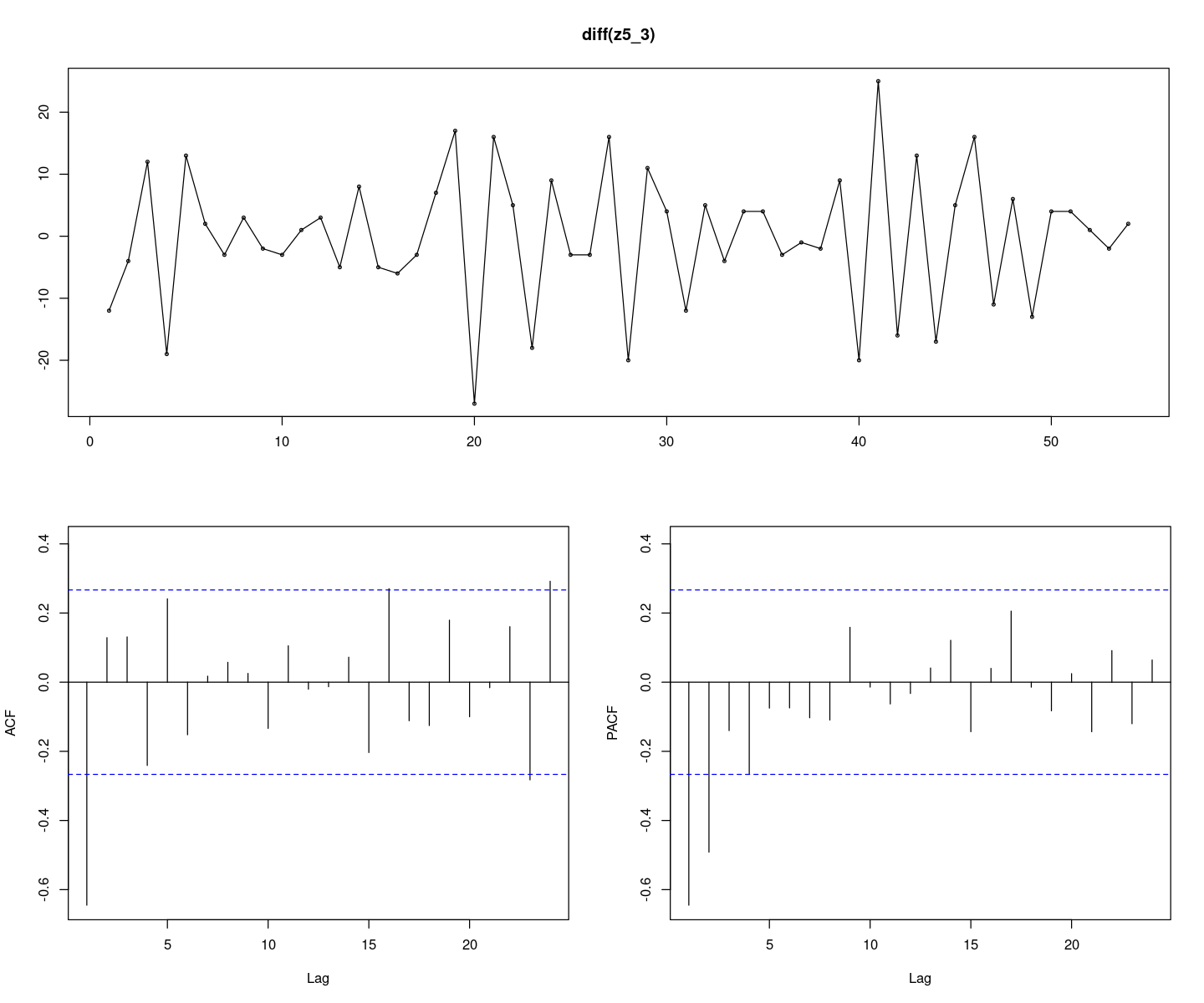
정상 시계열이다.
4번 문제와, 위의 결과로부터 차분의 순서에 대하여 논하라.
계절 성분을 먼저 차분 하면 추세가 없어지는 경우가 생기므로 그 이후의 차분을 하지 않아도 된다.
추세 차분을 먼저 하고 계절 차분을 진행해도 같은 정상 시계열을 얻을 수 있다. 다만, 모형이 복잡해질 수 있고 과대 차분으로 인해 분산이 커질 수 있다.
sd(z5_2)
sd(z5_3)옷! 근데 이 예제에서는 분산이 커지진 않는당 ㅎ
(R실습). ex8 2b.txt 는 어느 확률과정으로부터 생성된 모의시험 자료들이다. 각 자료를 가장 잘 설명하는 모형을 식별하고 추정한 후 잔차분석 포트맨토 검정 등의 모형 진단을 통해 모형을 적합하여라.
z6 <- scan("ex8_2b.txt")
forecast::tsdisplay(z6)
Registered S3 method overwritten by 'quantmod':
method from
as.zoo.data.frame zoo
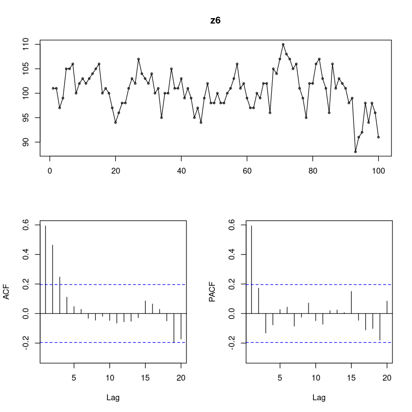
추세도 없고 계절성분도 없어 보인다. 정상 시계열!
ACF는 지수적으로 감소 PACF는 1차시 이후 감소 AR(1)모형이 적당해보인다.
#모형 적합도 검정 : H0 : rho1=...=rho_k=0 WN
Box.test(z6, lag=1, type = "Ljung-Box")
Box.test(z6, lag=6, type = "Ljung-Box")
Box.test(z6, lag=12, type = "Ljung-Box")
    Box-Ljung test

data:  z6
X-squared = 36.228, df = 1, p-value = 1.755e-09
    Box-Ljung test

data:  z6
X-squared = 66.617, df = 6, p-value = 2.015e-12
    Box-Ljung test

data:  z6
X-squared = 68.101, df = 12, p-value = 7.247e-10## 단위근 검정 H0 : 단위근이 있다.
fUnitRoots::adfTest(z6, lags = 0, type = "c")
fUnitRoots::adfTest(z6, lags = 1, type = "c")
fUnitRoots::adfTest(z6, lags = 2, type = "c")Warning message in fUnitRoots::adfTest(z6, lags = 0, type = "c"):
“p-value smaller than printed p-value”
Warning message in fUnitRoots::adfTest(z6, lags = 2, type = "c"):
“p-value smaller than printed p-value”
Title:
 Augmented Dickey-Fuller Test

Test Results:
  PARAMETER:
    Lag Order: 0
  STATISTIC:
    Dickey-Fuller: -4.469
  P VALUE:
    0.01

Description:
 Wed Nov 29 00:28:02 2023 by user:
Title:
 Augmented Dickey-Fuller Test

Test Results:
  PARAMETER:
    Lag Order: 1
  STATISTIC:
    Dickey-Fuller: -3.2151
  P VALUE:
    0.02306

Description:
 Wed Nov 29 00:28:02 2023 by user:
Title:
 Augmented Dickey-Fuller Test

Test Results:
  PARAMETER:
    Lag Order: 2
  STATISTIC:
    Dickey-Fuller: -3.5452
  P VALUE:
    0.01

Description:
Wed Nov 29 00:28:02 2023 by user: ## 모형적합 AR(1)
fit <- arima(z6,order=c(1,0,0))
summary(fit)
Call:
arima(x = z6, order = c(1, 0, 0))

Coefficients:
         ar1  intercept
      0.6231   100.4528
s.e.  0.0805     0.8253

sigma^2 estimated as 9.962:  log likelihood = -257.08,  aic = 520.16

Training set error measures:
                       ME     RMSE      MAE        MPE     MAPE      MASE
Training set -0.004602625 3.156255 2.452284 -0.1060461 2.457104 0.8991709
                  ACF1
Training set -0.100928ts.plot(z6, fitted(fit), col=1:2, lty=1:2, lwd=2)
abline(h=mean(z6), col="grey", lty=2)
legend("topleft", c("z6", "fitted z"), col=1:2, lty=1:2)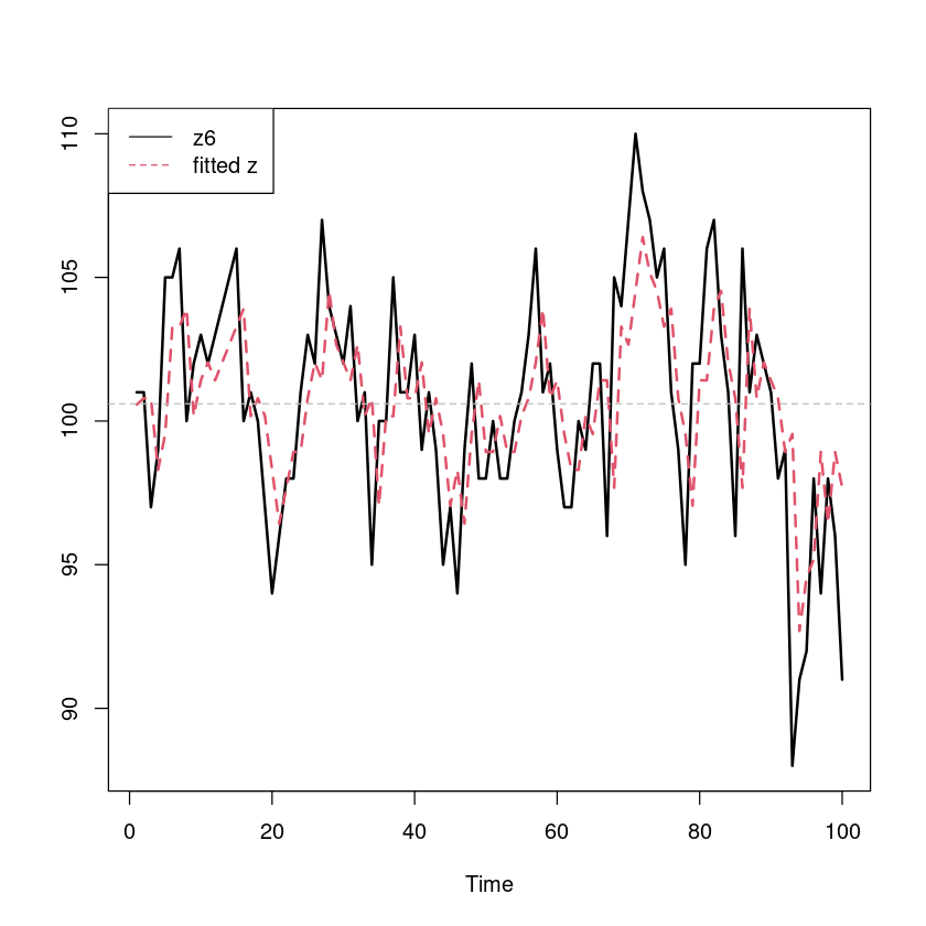
lmtest::coeftest(fit)
z test of coefficients:

           Estimate Std. Error  z value  Pr(>|z|)
ar1         0.62308    0.08054   7.7364 1.023e-14 ***
intercept 100.45278    0.82533 121.7118 < 2.2e-16 ***
---
Signif. codes:  0 ‘***’ 0.001 ‘**’ 0.01 ‘*’ 0.05 ‘.’ 0.1 ‘ ’ 1
모형: \((1-0.62308B)(Z_t - 100.45278) = \epsilon_t, \epsilon_t \sim WN(0, 9.926)\)
fit$sigma2즉 모형은 AR(1)모형이고
\(Z_t − 100.45278 = - 0.62308(Z_{t−1} − 100.45278) + ε_t\)
\(\hatσ^2 = 9.96194659591476\)
- 모형진단
- 잔차분석
resid = resid(fit)
forecast::tsdisplay(resid)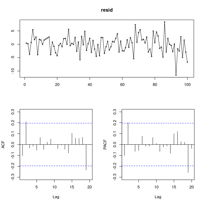
- ACF가 2시차에서 살짝 유의해 보인다.. –> MA(2)모형이 추가 될지도?
# 잔차의 포트맨토 검정 ## H0 : rho1=...=rho_k=0
portes::LjungBox(fit, lags=c(6,12,18,24))| lags | statistic | df | p-value | |
|---|---|---|---|---|
| 6 | 6.515031 | 5 | 0.2592767 | |
| 12 | 7.252215 | 11 | 0.7783062 | |
| 18 | 10.891994 | 17 | 0.8621232 | |
| 24 | 20.207804 | 23 | 0.6293457 |
- Box.test를 진행할 때 residual을 사용하는 경우 fitdf=p+q옵션을 꼭 넣어야 한다.
- AR(1)이므로 p+q=1
#모형 적합도 검정 : H0 : rho1=...=rho_k=0 WN
Box.test(resid(fit), lag=2, type = "Ljung-Box", fitdf=1)
Box.test(resid(fit), lag=6, type = "Ljung-Box", fitdf=1)
Box.test(resid(fit), lag=12, type = "Ljung-Box", fitdf=1)
## 정규성검정
tseries::jarque.bera.test(resid) ##JB test H0: norma
    Jarque Bera Test

data:  resid
X-squared = 5.6073, df = 2, p-value = 0.06059par(mfrow=c(1,2))
hist(resid)
qqnorm(resid, pch=16)
qqline(resid)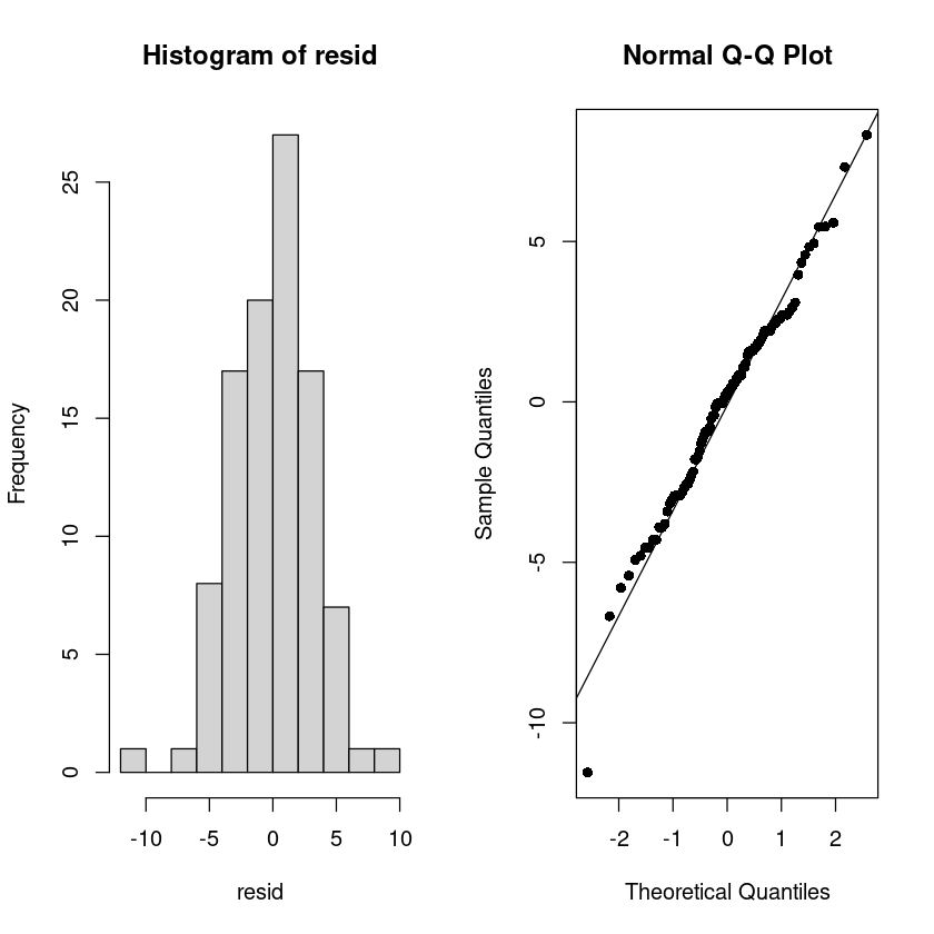
## 잔차 검정
astsa::sarima(z6, p=1, d=0, q=0)
initial value 1.388134
iter 2 value 1.155478
iter 3 value 1.154827
iter 4 value 1.154367
iter 5 value 1.154330
iter 6 value 1.154281
iter 7 value 1.154281
iter 8 value 1.154281
iter 9 value 1.154281
iter 10 value 1.154281
iter 10 value 1.154281
iter 10 value 1.154281
final value 1.154281
converged
initial value 1.151883
iter 2 value 1.151854
iter 3 value 1.151845
iter 4 value 1.151844
iter 5 value 1.151843
iter 5 value 1.151843
iter 5 value 1.151843
final value 1.151843
converged$fit
Call:
arima(x = xdata, order = c(p, d, q), seasonal = list(order = c(P, D, Q), period = S),
xreg = xmean, include.mean = FALSE, transform.pars = trans, fixed = fixed,
optim.control = list(trace = trc, REPORT = 1, reltol = tol))
Coefficients:
ar1 xmean
0.6231 100.4528
s.e. 0.0805 0.8253
sigma^2 estimated as 9.962: log likelihood = -257.08, aic = 520.16
$degrees_of_freedom
[1] 98
$ttable
Estimate SE t.value p.value
ar1 0.6231 0.0805 7.7364 0
xmean 100.4528 0.8253 121.7118 0
$AIC
[1] 5.201564
$AICc
[1] 5.202801
$BIC
[1] 5.279719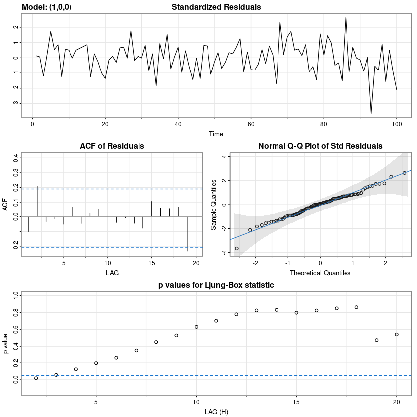
- 과대적합
fit1 <- arima(z6,order=c(1,0,0)) #AR(1)
fit2 <- arima(z6,order=c(2,0,0)) #AR(2)
fit3 <- arima(z6,order=c(1,0,1)) #ARMA(1,1)lmtest::coeftest(fit1)
z test of coefficients:

           Estimate Std. Error  z value  Pr(>|z|)
ar1         0.62308    0.08054   7.7364 1.023e-14 ***
intercept 100.45278    0.82533 121.7118 < 2.2e-16 ***
---
Signif. codes: 0 ‘***’ 0.001 ‘**’ 0.01 ‘*’ 0.05 ‘.’ 0.1 ‘ ’ 1lmtest::coeftest(fit2)
z test of coefficients:

            Estimate Std. Error  z value  Pr(>|z|)
ar1         0.514525   0.099785   5.1564 2.518e-07 ***
ar2         0.178841   0.100295   1.7832   0.07456 .
intercept 100.380132   0.989402 101.4554 < 2.2e-16 ***
---
Signif. codes: 0 ‘***’ 0.001 ‘**’ 0.01 ‘*’ 0.05 ‘.’ 0.1 ‘ ’ 1lmtest::coeftest(fit3)
z test of coefficients:

            Estimate Std. Error  z value  Pr(>|z|)
ar1         0.738491   0.096895   7.6215 2.507e-14 ***
ma1        -0.183319   0.125867  -1.4565    0.1453
intercept 100.392697   0.955466 105.0719 < 2.2e-16 ***
---
Signif. codes: 0 ‘***’ 0.001 ‘**’ 0.01 ‘*’ 0.05 ‘.’ 0.1 ‘ ’ 1paste0("AIC for AR(1) = ", fit1$aic)
paste0("AIC for AR(2) = ", fit2$aic)
paste0("AIC for ARMA(1,1) = ", fit3$aic)# 올바르게 선택했는지 확인용
forecast::auto.arima(z6, trace = T)
 ARIMA(2,0,2) with non-zero mean : 520.8564
 ARIMA(0,0,0) with non-zero mean : 564.5433
 ARIMA(1,0,0) with non-zero mean : 520.4064
 ARIMA(0,0,1) with non-zero mean : 539.802
 ARIMA(0,0,0) with zero mean     : 1208.216
 ARIMA(2,0,0) with non-zero mean : 519.4539
 ARIMA(3,0,0) with non-zero mean : 519.4331
 ARIMA(4,0,0) with non-zero mean : 521.4544
 ARIMA(3,0,1) with non-zero mean : 521.5667
 ARIMA(2,0,1) with non-zero mean : 520.4177
 ARIMA(4,0,1) with non-zero mean : 523.7179
 ARIMA(3,0,0) with zero mean     : Inf

 Best model: ARIMA(3,0,0) with non-zero mean
Series: z6
ARIMA(3,0,0) with non-zero mean

Coefficients:
         ar1     ar2      ar3      mean
      0.5428  0.2545  -0.1524  100.4523
s.e.  0.1003  0.1110   0.1012    0.8540

sigma^2 = 9.822:  log likelihood = -254.4
AIC=518.79   AICc=519.43   BIC=531.82
fit4 <- arima(z6,order=c(3,0,0)) #AR(3)
lmtest::coeftest(fit4)
z test of coefficients:

           Estimate Std. Error  z value  Pr(>|z|)
ar1         0.54278    0.10028   5.4125 6.214e-08 ***
ar2         0.25451    0.11103   2.2923   0.02189 *
ar3        -0.15237    0.10121  -1.5054   0.13221
intercept 100.45229    0.85397 117.6303 < 2.2e-16 ***
---
Signif. codes:  0 ‘***’ 0.001 ‘**’ 0.01 ‘*’ 0.05 ‘.’ 0.1 ‘ ’ 1
(best로 뽑아준거 AR(3)이 AR(1)보다는 나아 보이지 않는다. .. 모형이 덜 복잡한 AR(1)모형 선택)
교수님은 ARMA(1,2)모형을 선택함
(R실습). ex7 5c.txt 는 어느 확률과정으로부터 생성된 모의시험 자료들이다. 각 자료를 가장 잘 설명하는 모형을 식별하고 추정한 후 잔차분석 포트맨토 검정 등의 모형 진단을 통해 모형을 적합하여라.
z7 <- scan("ex7_5c.txt")
forecast::tsdisplay(z7)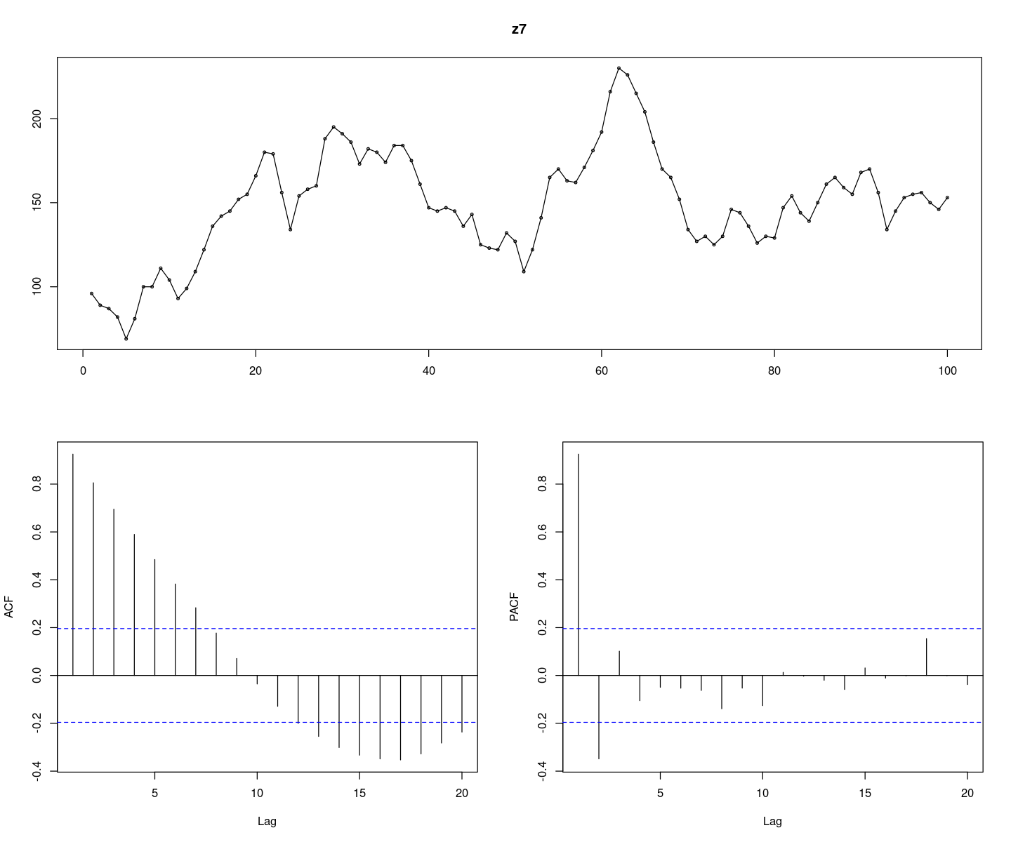
확률적 추세가 있어보인다.
acf(z7, lag.max=100)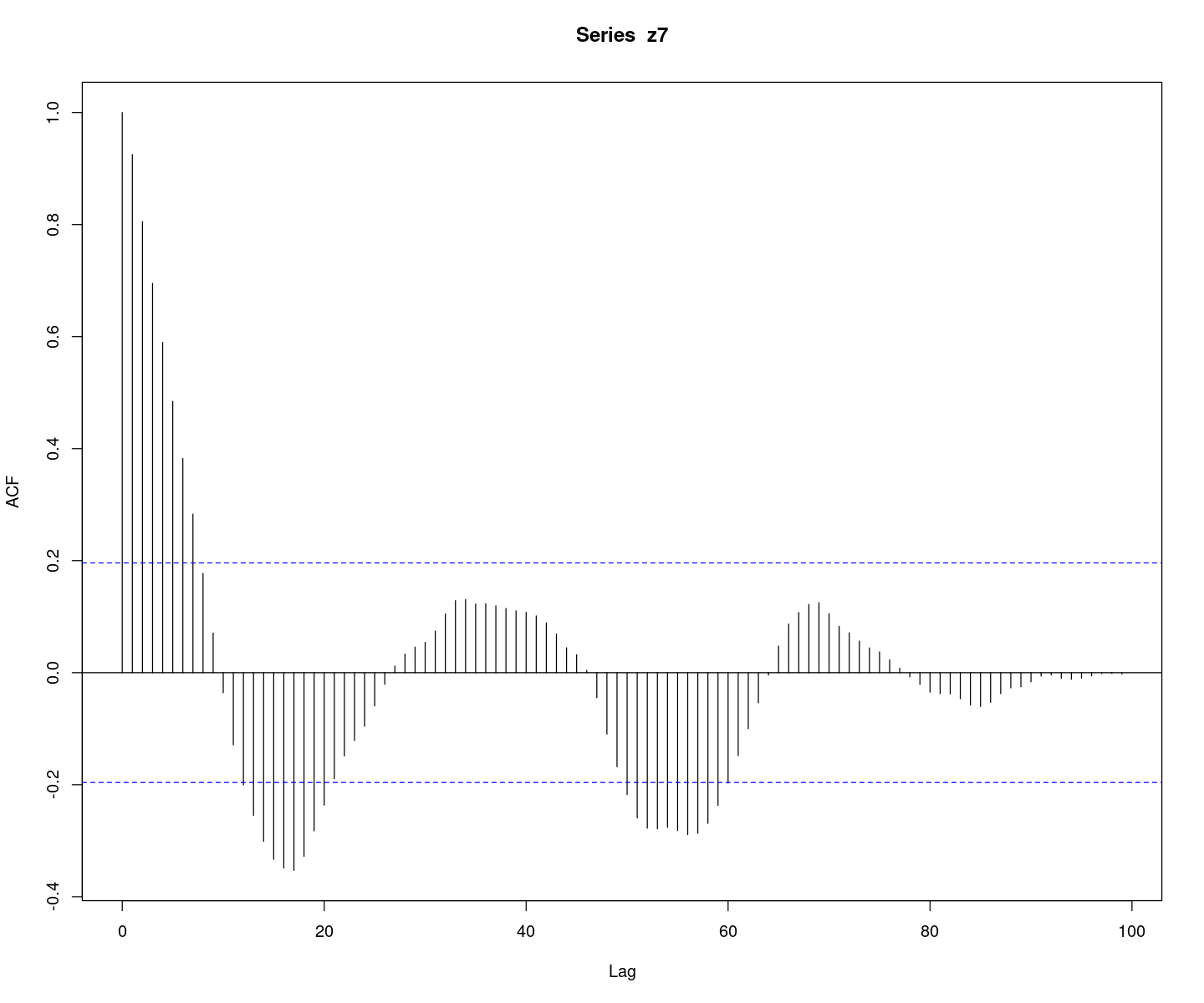
pacf(z7, lag.max=100)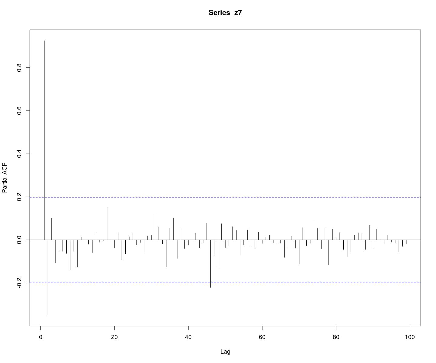
추세가 있어보이나.. 결정적 추세가 아닌 확률적 추세가 있어보인다. 평균이 100근처인 느낌이다.
ACF가 그림상 sin함수의 주기로 감소하는 느낌…. pacf는 2개만 살아있고 다 절단이다. AR(2)모형인 것 같다.
#모형 적합도 검정 : H0 : rho1=...=rho_k=0 WN
Box.test(z7, lag=1, type = "Ljung-Box")
Box.test(z7, lag=6, type = "Ljung-Box")
Box.test(z7, lag=12, type = "Ljung-Box")
    Box-Ljung test

data:  z7
X-squared = 88.163, df = 1, p-value < 2.2e-16
    Box-Ljung test

data:  z7
X-squared = 284.49, df = 6, p-value < 2.2e-16
    Box-Ljung test

data:  z7
X-squared = 304.02, df = 12, p-value < 2.2e-16tseries::adf.test(z7) # ADF 검정
## 단위근 검정 H0 : 단위근이 있다.
    Augmented Dickey-Fuller Test

data:  z7
Dickey-Fuller = -2.9537, Lag order = 4, p-value = 0.1816
alternative hypothesis: stationarytseries::pp.test(z7) # PP 검정
    Phillips-Perron Unit Root Test

data:  z7
Dickey-Fuller Z(alpha) = -10.033, Truncation lag parameter = 3, p-value
= 0.5337
alternative hypothesis: stationary결정적 추세가 아닌 확률적 추세가 있어보이므로 차분을 진행하자.
- adfTest에서 lag는 단위근을 검정하기 위해 가정하는 모형이 AR차수인데, 미리 결정을 해야하는 것이다.
- 하지만 미리 모형을 적합하기 전까지는 알 수가 없으므로 여러 개 해보면 된다.
- lag=0,2에서 기각을 하지 못했으니 차분이 필요하다.
## 차분
diff_z = diff(z7)
forecast::tsdisplay(diff_z)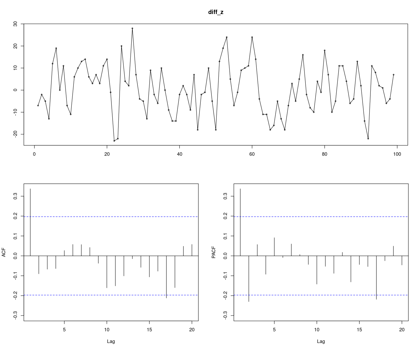
- 정상시계열로 보인다.
- ACF는 1차 이후 절단, PACF는 2차 이후 절단이므로 MA(1)모형 선택
- 원래 데이터에 대해 ARIMA(0,1,1)모형 적합
- \((1-B)Z_T = (1-\theta)\epsilon_t, \epsilon_t \sim WN(0,\sigma^2)\)
Box.test(diff(z7), lag=6, type = "Ljung-Box")
Box.test(diff(z7), lag=12, type = "Ljung-Box")
    Box-Ljung test

data:  diff(z7)
X-squared = 13.76, df = 6, p-value = 0.03244
    Box-Ljung test

data:  diff(z7)
X-squared = 21.112, df = 12, p-value = 0.04876t.test(diff(z7))
    One Sample t-test

data:  diff(z7)
t = 0.51483, df = 98, p-value = 0.6078
alternative hypothesis: true mean is not equal to 0
95 percent confidence interval:
 -1.643556  2.795071
sample estimates:
mean of x
0.5757576 fit <- arima(z7, order=c(0,1,1))
fit- 추정된 계수가 유의하므로 후보모형으로 선정
- \((1-B)Z_t = (1+0.4905B)\epsilon_t, \epsilon_t \sim WN(0,102.2)\)
- 진단
forecast::checkresiduals(fit)# Zt ~ radomwalk, ARIMA(0,1,0) with drift
## 모형 ARIMA(0,1,0)
fit <- arima(z7,order=c(0,1,0))
summary(fit)
Call:
arima(x = z7, order = c(0, 1, 0))


sigma^2 estimated as 122.9:  log likelihood = -378.64,  aic = 759.27

Training set error measures:
                  ME     RMSE     MAE      MPE     MAPE      MASE      ACF1
Training set 0.57096 11.03042 9.03096 0.157609 6.319408 0.9901052 0.3373427
- 분해법 이용
################################
## 회귀모형
t <- 1:length(z7)
fit1 <- lm(z7~t)
summary(fit1)
Call:
lm(formula = z7 ~ t)

Residuals:
    Min      1Q  Median      3Q     Max
-63.730 -22.451  -4.656  18.260  77.126

Coefficients:
            Estimate Std. Error t value Pr(>|t|)
(Intercept) 130.9630     6.0886  21.510  < 2e-16 ***
t             0.3534     0.1047   3.376  0.00105 **
---
Signif. codes:  0 ‘***’ 0.001 ‘**’ 0.01 ‘*’ 0.05 ‘.’ 0.1 ‘ ’ 1

Residual standard error: 30.21 on 98 degrees of freedom
Multiple R-squared:  0.1042,    Adjusted R-squared:  0.09506
F-statistic:  11.4 on 1 and 98 DF,  p-value: 0.001055
\(\hat T_t = 130.9630 + 0.3534 t\)
\(Z_t = T_t + I_t = b_0 + b_1t + e_t\)
et <- z7 - fitted(fit1) #추세 제거
forecast::tsdisplay(et, main="추세 제거 e7")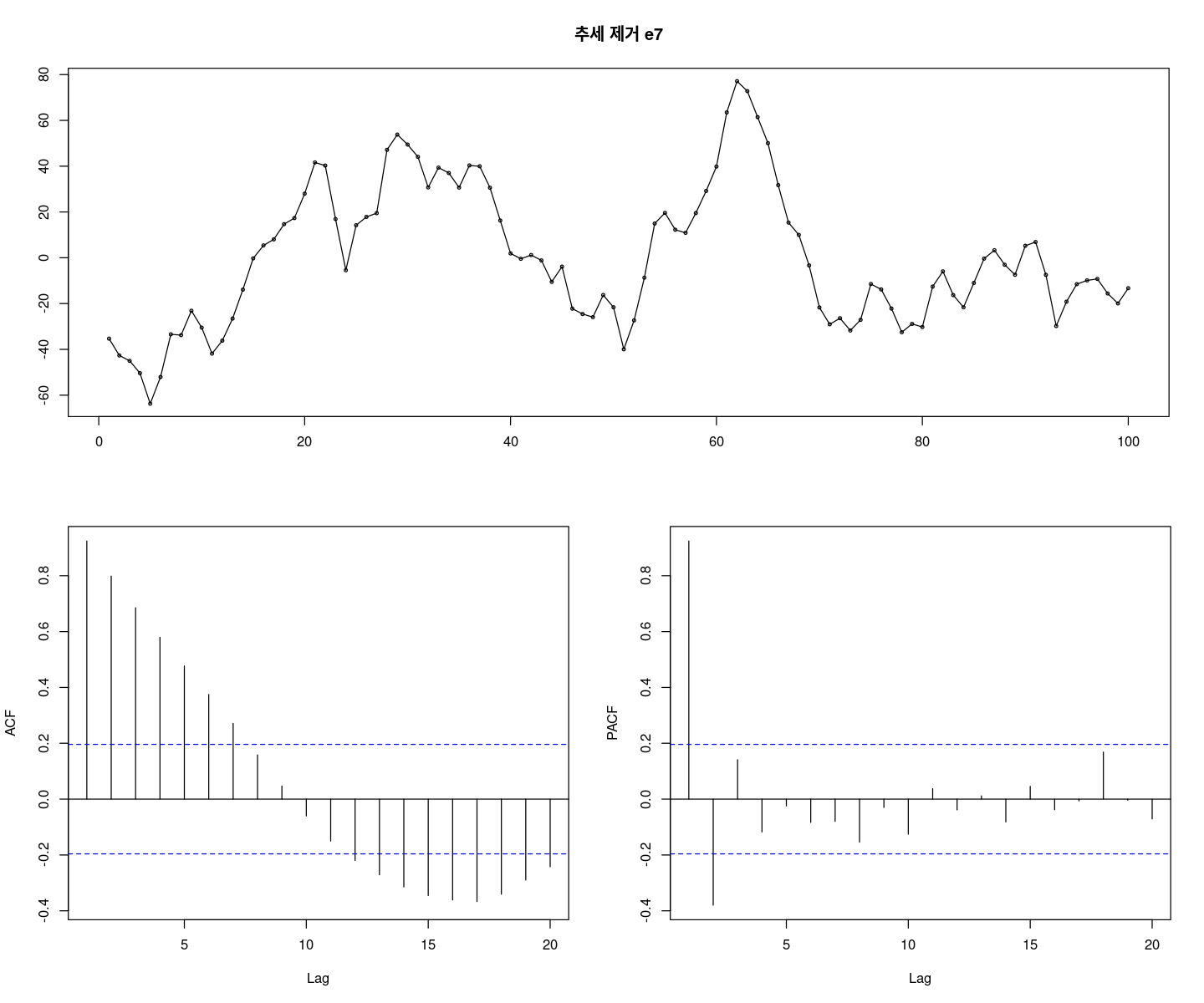
# 모형 적합도 확인
##H0 : rho1 = ... = rho6 = 0
Box.test(et, lag=6, type = "Ljung-Box")
##H0 : rho1 = ... = rho12 = 0
Box.test(et, lag=12, type = "Ljung-Box")
    Box-Ljung test

data:  et
X-squared = 279.09, df = 6, p-value < 2.2e-16
    Box-Ljung test

data:  et
X-squared = 298.76, df = 12, p-value < 2.2e-16#H0 : phi=1
fUnitRoots::adfTest(et, lags = 0, type = "nc")
fUnitRoots::adfTest(et, lags = 1, type = "nc")
fUnitRoots::adfTest(et, lags = 2, type = "nc")
Title:
 Augmented Dickey-Fuller Test

Test Results:
  PARAMETER:
    Lag Order: 0
  STATISTIC:
    Dickey-Fuller: -2.0272
  P VALUE:
    0.04335

Description:
 Wed Nov 29 22:15:48 2023 by user:
Warning message in fUnitRoots::adfTest(et, lags = 1, type = "nc"):
“p-value smaller than printed p-value”
Title:
 Augmented Dickey-Fuller Test

Test Results:
  PARAMETER:
    Lag Order: 1
  STATISTIC:
    Dickey-Fuller: -2.9693
  P VALUE:
    0.01

Description:
 Wed Nov 29 22:15:48 2023 by user:
Title:
 Augmented Dickey-Fuller Test

Test Results:
  PARAMETER:
    Lag Order: 2
  STATISTIC:
    Dickey-Fuller: -2.4681
  P VALUE:
    0.01551

Description:
Wed Nov 29 22:15:48 2023 by user: t.test(et)
    One Sample t-test

data:  et
t = -6.6103e-16, df = 99, p-value = 1
alternative hypothesis: true mean is not equal to 0
95 percent confidence interval:
 -5.964947  5.964947
sample estimates:
    mean of x
-1.987195e-15
###### lm (1차추세 모형)
###### et ~ AR(2)
fit_et <- arima(et, order=c(2,0,0),
include.mean = F) ## et
summary(fit_et)
Call:
arima(x = et, order = c(2, 0, 0), include.mean = F)

Coefficients:
         ar1      ar2
      1.2897  -0.3875
s.e.  0.0913   0.0923

sigma^2 estimated as 100.3:  log likelihood = -373.45,  aic = 752.9

Training set error measures:
                     ME     RMSE    MAE       MPE    MAPE      MASE       ACF1
Training set 0.07085178 10.01366 7.9766 -35.02261 105.705 0.8734854 0.06942246
\(z_t = 1.2897⋅z_{t−1} −0.3875⋅z_{t−2}+ϵ_t\)
1.2897-0.3875lmtest::coeftest(fit_et)
z test of coefficients:

     Estimate Std. Error z value  Pr(>|z|)
ar1  1.289702   0.091293 14.1270 < 2.2e-16 ***
ar2 -0.387540   0.092268 -4.2002 2.667e-05 ***
---
Signif. codes:  0 ‘***’ 0.001 ‘**’ 0.01 ‘*’ 0.05 ‘.’ 0.1 ‘ ’ 1
유의하네…
#hat_zt = hat_Tt + hat_et
hat_zt = fitted(fit1) + fitted(fit_et)
ts.plot(z7, hat_zt, col=1:2, lty=1:2, lwd=2)
legend("topleft", c("z7","hat_z"), col=1:2, lty=1:2, lwd=2)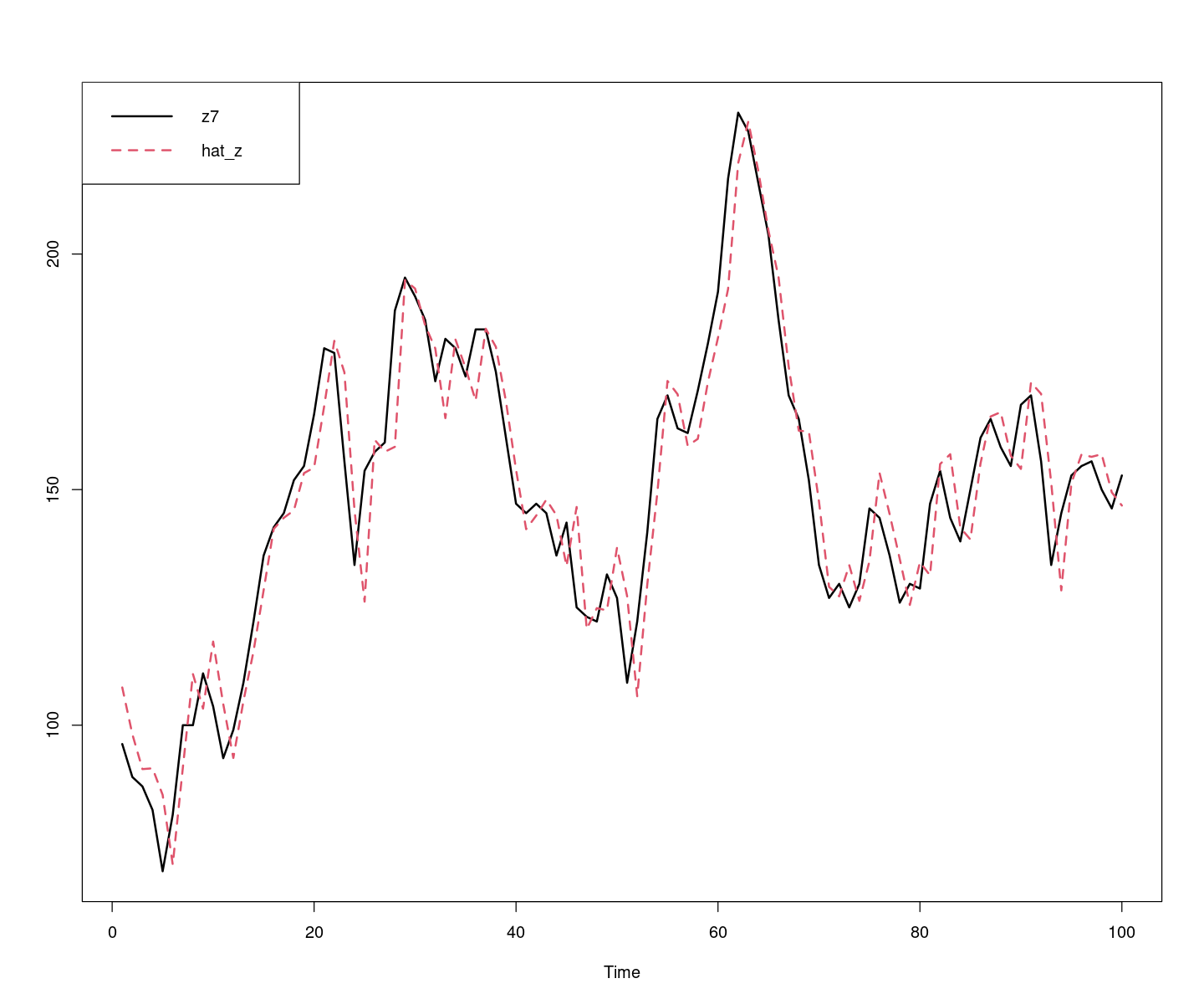
#### ut에 대한 잔차검정
ut <- resid(fit_et)
forecast::tsdisplay(ut)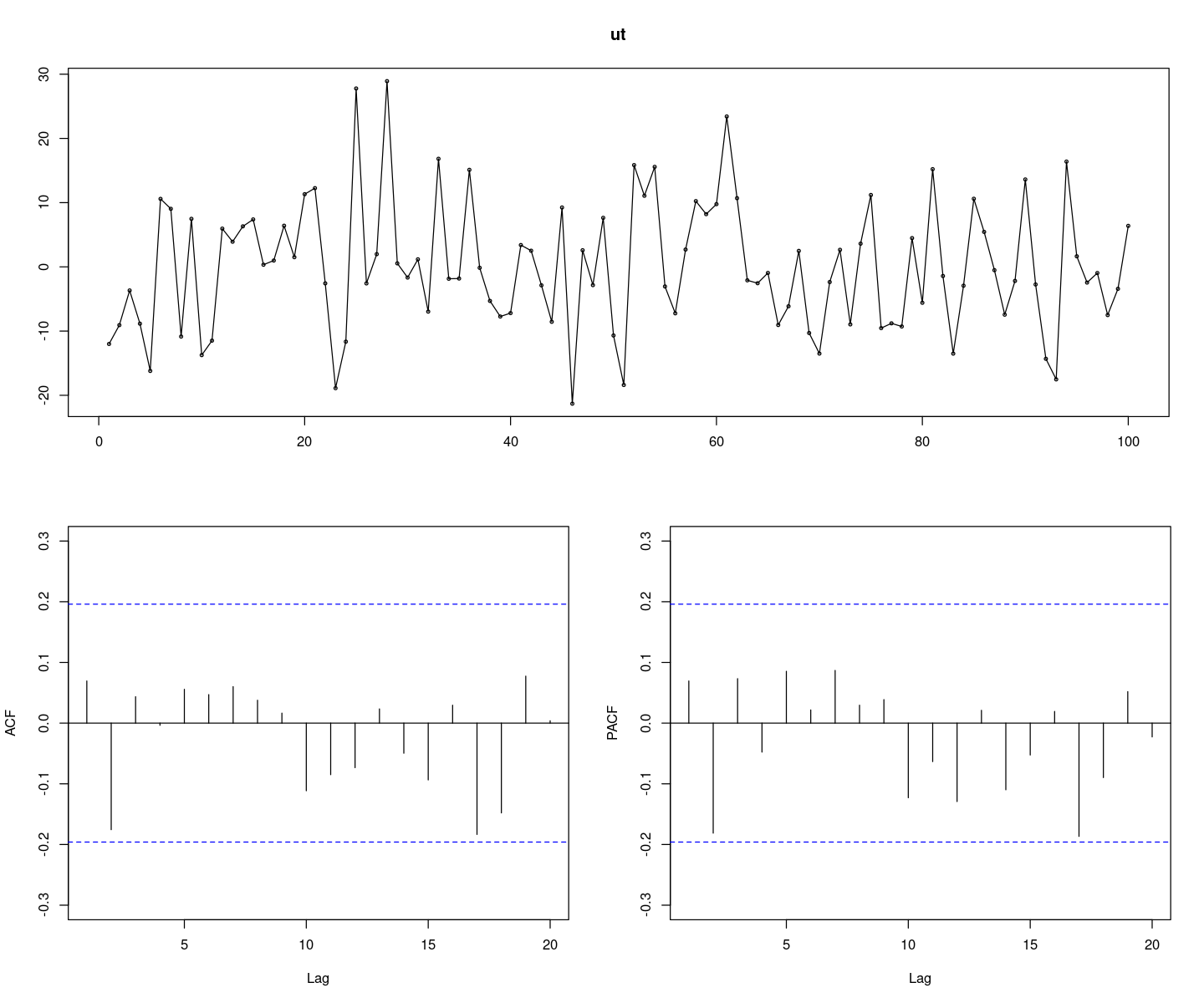
## 정규성검정
tseries::jarque.bera.test(ut) ##JB test H0: normal
    Jarque Bera Test

data:  ut
X-squared = 2.5243, df = 2, p-value = 0.283par(mfrow=c(1,2))
hist(ut)
qqnorm(ut, pch=16)
qqline(ut)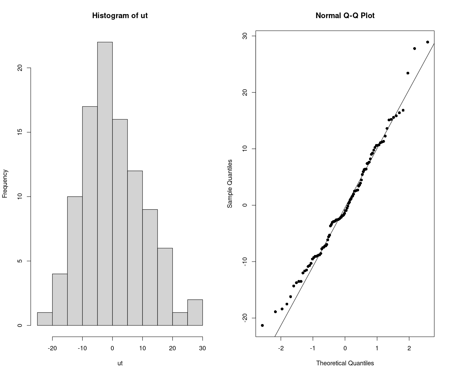
# 잔차의 포트맨토 검정 ## H0 : rho1=...=rho_k=0
portes::LjungBox(fit_et, lags=c(6,12,18,24))| lags | statistic | df | p-value | |
|---|---|---|---|---|
| 6 | 4.478742 | 4 | 0.3450755 | |
| 12 | 7.922301 | 10 | 0.6364264 | |
| 18 | 16.292465 | 16 | 0.4327419 | |
| 24 | 18.569598 | 22 | 0.6717336 |
## 잔차 검정
astsa::sarima(et, p=2, d=0, q=0)
initial value 3.390891
iter 2 value 3.366724
iter 3 value 2.566255
iter 4 value 2.445142
iter 5 value 2.325612
iter 6 value 2.303803
iter 7 value 2.302399
iter 8 value 2.302221
iter 9 value 2.302187
iter 10 value 2.302174
iter 11 value 2.302142
iter 12 value 2.302121
iter 13 value 2.302100
iter 14 value 2.302097
iter 15 value 2.302097
iter 15 value 2.302097
final value 2.302097
converged
initial value 2.316698
iter 2 value 2.316354
iter 3 value 2.315707
iter 4 value 2.315565
iter 5 value 2.315436
iter 6 value 2.315391
iter 7 value 2.315378
iter 8 value 2.315377
iter 8 value 2.315377
final value 2.315377
converged$fit
Call:
arima(x = xdata, order = c(p, d, q), seasonal = list(order = c(P, D, Q), period = S),
xreg = xmean, include.mean = FALSE, transform.pars = trans, fixed = fixed,
optim.control = list(trace = trc, REPORT = 1, reltol = tol))
Coefficients:
ar1 ar2 xmean
1.2889 -0.3866 -1.8345
s.e. 0.0914 0.0924 9.7931
sigma^2 estimated as 100.2: log likelihood = -373.43, aic = 754.86
$degrees_of_freedom
[1] 97
$ttable
Estimate SE t.value p.value
ar1 1.2889 0.0914 14.1042 0.0000
ar2 -0.3866 0.0924 -4.1843 0.0001
xmean -1.8345 9.7931 -0.1873 0.8518
$AIC
[1] 7.548632
$AICc
[1] 7.551132
$BIC
[1] 7.652838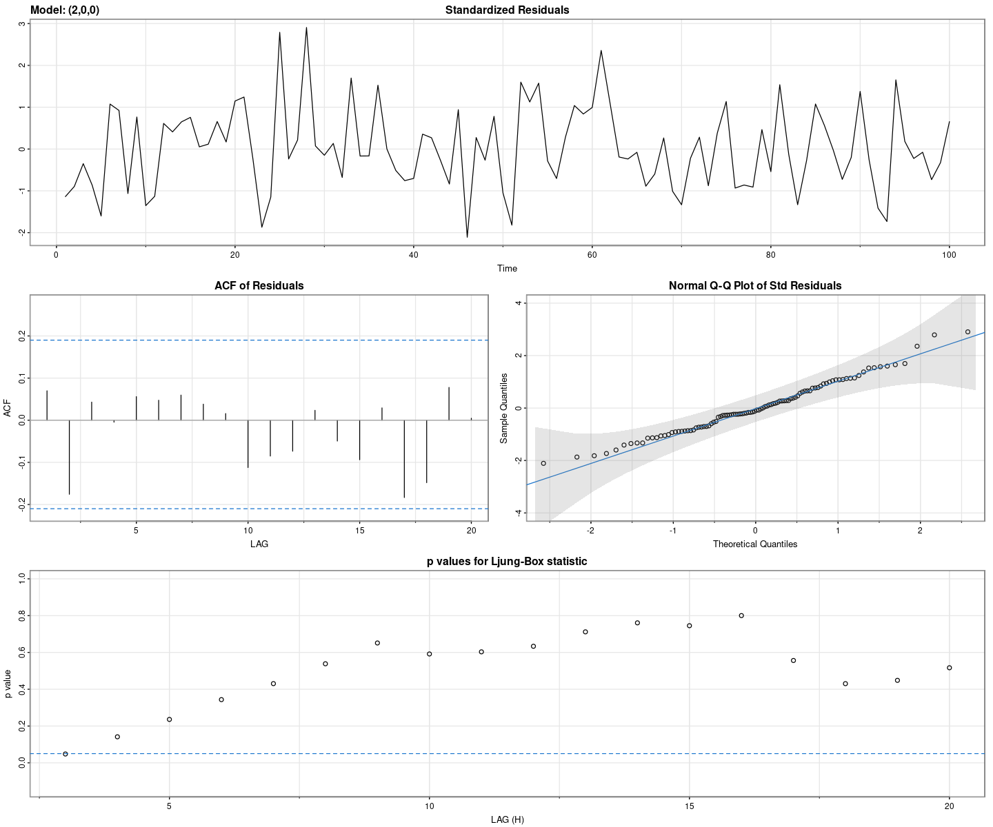
# 올바르게 선택했는지 확인용
forecast::auto.arima(z7, trace = T)
 ARIMA(2,1,2) with drift         : Inf
 ARIMA(0,1,0) with drift         : 761.1324
 ARIMA(1,1,0) with drift         : 751.3387
 ARIMA(0,1,1) with drift         : 745.3847
 ARIMA(0,1,0)                    : 759.316
 ARIMA(1,1,1) with drift         : 746.6741
 ARIMA(0,1,2) with drift         : 746.685
 ARIMA(1,1,2) with drift         : 748.8309
 ARIMA(0,1,1)                    : 743.4057
 ARIMA(1,1,1)                    : 744.6798
 ARIMA(0,1,2)                    : 744.6976
 ARIMA(1,1,0)                    : 749.3425
 ARIMA(1,1,2)                    : 746.8224

 Best model: ARIMA(0,1,1)
Series: z7
ARIMA(0,1,1)

Coefficients:
         ma1
      0.4905
s.e.  0.0986

sigma^2 = 103.2:  log likelihood = -369.64
AIC=743.28   AICc=743.41   BIC=748.47